APIs & Interactive Maps with Leaflet in R
Today I made my first API requests in R! Using the Open Notify API, I pulled the information of when the International Space Station (ISS) is scheduled to pass over United States state capitals then mapped them using {leaflet}. This exercise is part of lab 3 in the curriculum of Cal Poly’s Stat 431.
This Open-Notify API provides predictions of pass times for a given location when given the corresponding latitude and longitude.
U.S. State Captials Information
To get the latitudes and longitudes of US state capitals, I used this resource.
library(tidyverse)
library(httr)     ## for working with the API
library(jsonlite) ## to work with the JSON data

# Get the long & lats of all the US state capitals
capitals <- read.table("https://people.sc.fsu.edu/~jburkardt/datasets/states/state_capitals_ll.txt", col.names = c("state","latitude","longitude"))

# Get the state capital names
capital_names <- read.table("https://people.sc.fsu.edu/~jburkardt/datasets/states/state_capitals_name.txt", col.names = c("state","capital"))

capitals <- bind_cols(capitals, capital_names)| state | latitude | longitude | state1 | capital |
|---|---|---|---|---|
| AL | 32.36154 | -86.27912 | AL | Montgomery |
| AK | 58.30194 | -134.41974 | AK | Juneau |
| AZ | 33.44846 | -112.07384 | AZ | Phoenix |
| AR | 34.73601 | -92.33112 | AR | Little Rock |
| CA | 38.55560 | -121.46893 | CA | Sacramento |
Pass Times for U.S. State Captials
After getting the capitals information, I requested the ISS data from the Open Notify API. To see the structure of the response and how to get the information I needed, I looked at the information for one capital first.
# Getting the data for the first state
response <- GET("http://api.open-notify.org/iss-pass.json", query = list(lat = capitals$latitude[1], lon = capitals$longitude[1]))

# Extract the data from the response
data = fromJSON(rawToChar(response$content))

# Looking at the first pass time
data$response[1,]
## duration risetime
## 1 640 1591235377# Convert unix time to datetime
as.POSIXct(as.numeric(data$response[1,][2]), origin="1970-01-01")## [1] "2020-06-03 18:49:37 PDT"Now that I knew the structure of the data, I iterated the process of requesting the next three pass times from the API for each state capital.
# Initialize dataframe
capitals_pass_times <- tibble(state = character(),
       capital = character(),
       lat = numeric(),
       lon = numeric(),
       duration = numeric(),
       risetime_num = character(),
       risetime = numeric())

# Loop for all states
for (s in 1:nrow(capitals)) {
  # Getting the data for the first state
  response <- GET("http://api.open-notify.org/iss-pass.json", query = list(lat = capitals$latitude[s], lon = capitals$longitude[s]))
  # Extract the data from the response
  data = fromJSON(rawToChar(response$content))

  # Add the next 3 predicted pass times to dataframe
  for (i in 1:3) {
  capitals_pass_times <- capitals_pass_times %>% add_row(state = capitals$state[s],
       capital = capitals$capital[s],
       lat = capitals$latitude[s],
       lon = capitals$longitude[s],
       duration = as.numeric(data$response[i,]["duration"]),
       risetime_num = paste0("risetime_",i),
       risetime = as.numeric(data$response[i,]["risetime"]))
  }
}| state | capital | lat | lon | duration | risetime_num | risetime |
|---|---|---|---|---|---|---|
| AL | Montgomery | 32.36154 | -86.27912 | 640 | risetime_1 | 1591235377 |
| AL | Montgomery | 32.36154 | -86.27912 | 563 | risetime_2 | 1591241207 |
| AL | Montgomery | 32.36154 | -86.27912 | 537 | risetime_3 | 1591289620 |
| AK | Juneau | 58.30194 | -134.41974 | 619 | risetime_1 | 1591234747 |
| AK | Juneau | 58.30194 | -134.41974 | 587 | risetime_2 | 1591240530 |
| AK | Juneau | 58.30194 | -134.41974 | 437 | risetime_3 | 1591246349 |
Mapping the Capitals & Displaying the Pass Times
Using the {leaflet} package, I made a map with the US state capitals showing the next three predicted pass times for each capital. When hovering over a capital, the next predicted pass time will show. When clicking a capital, you’ll be able to see the next three predicted pass times.
library(leaflet)
# Pivot table
capitals_pass_times <- pivot_wider(capitals_pass_times, id_cols = c(state,capital,lat,lon), names_from = risetime_num, values_from = risetime)
# Convert unix time to datetime
capitals_pass_times <- capitals_pass_times %>%
mutate_at(c("risetime_1", "risetime_2", "risetime_3"), ~as.POSIXct(., origin="1970-01-01")) %>%
arrange(risetime_1)
# Get ISS icon
ISSicon <- makeIcon(iconUrl = "http://open-notify.org/Open-Notify-API/map/ISSIcon.png",
iconWidth = 15, iconHeight = 15)
# Map with leaflet
m <- leaflet(data = capitals_pass_times) %>%
addTiles() %>% # Add default OpenStreetMap map tiles
addMarkers(lng = ~lon, lat = ~lat,
label = paste0(capitals_pass_times$capital, ", ", capitals_pass_times$state, " - Next predicted passtime: ", capitals_pass_times$risetime_1),
popup = paste0(capitals_pass_times$capital, ", ", capitals_pass_times$state, " - Next predicted passtimes: ", capitals_pass_times$risetime_1, ", ", capitals_pass_times$risetime_2, ", ", capitals_pass_times$risetime_3),
icon = ISSicon)
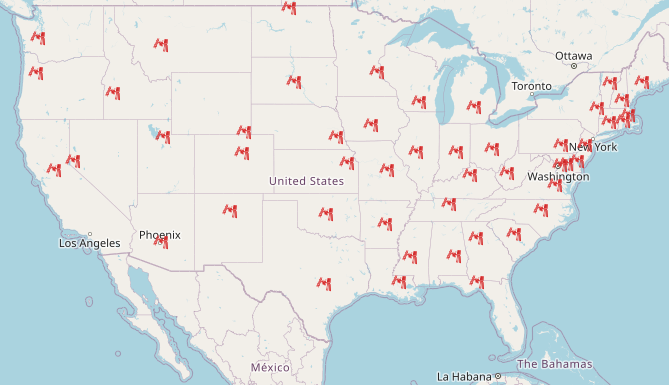
mDrawing the Route of the ISS
To see the expected pass order of the ISS, I added polylines in order of pass times.
route <- leaflet(data = capitals_pass_times) %>%
  addTiles() %>%  # Add default OpenStreetMap map tiles
  addPolylines(lat = ~lat, lng = ~lon, color = "red") %>%
  addMarkers(lng = ~lon, lat = ~lat,
             label = paste0(capitals_pass_times$capital, ", ",  capitals_pass_times$state, " - Next predicted passtime: ", capitals_pass_times$risetime_1),
             popup = paste0(capitals_pass_times$capital, ", ",  capitals_pass_times$state,  " - Next predicted passtimes: ", capitals_pass_times$risetime_1, ", ", capitals_pass_times$risetime_2, ", ", capitals_pass_times$risetime_3),
             icon = ISSicon)

route